Level: Medium. Analyze differential voltage variation in a resistive bridge by modifying a sensor.
Objective and use case
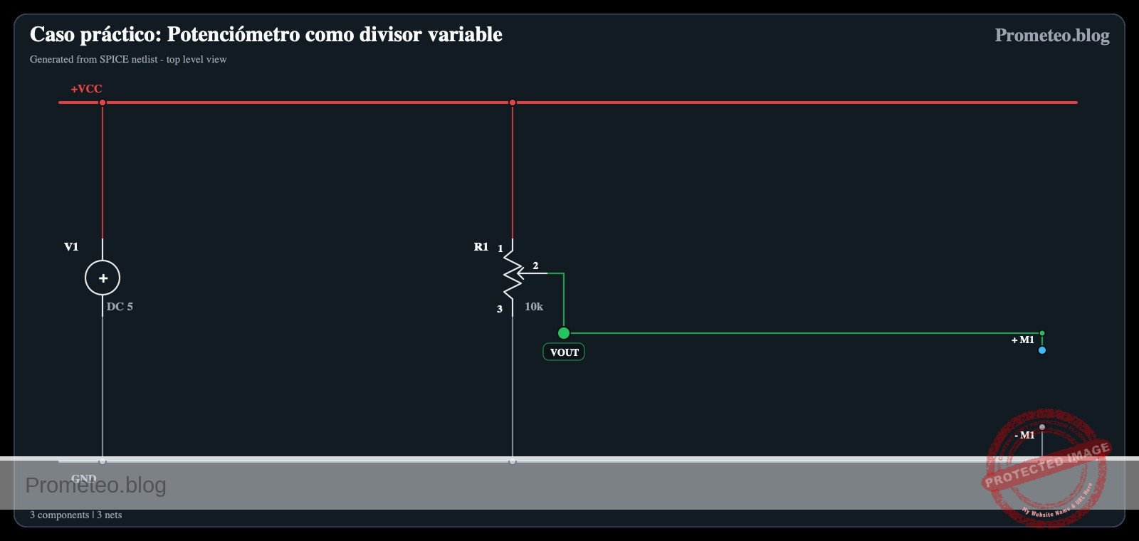
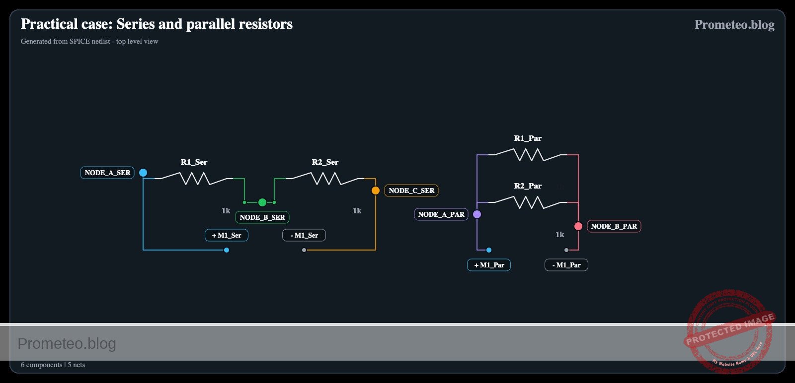
You will build a Wheatstone bridge circuit using three fixed resistors and one variable resistor to simulate a resistive sensor. This circuit converts a change in resistance into a measurable differential voltage output.
Why it is useful:
* Precision Sensing: Used in load cells (weighing scales) and strain gauges where resistance changes are minute.
* Temperature Measurement: Fundamental for reading RTDs (Resistance Temperature Detectors) and thermistors.
* Zero Calibration: Allows systems to establish a «null point» (0 V output) to cancel out offset errors before taking measurements.
* Small Signal Detection: Filters out power supply noise common to both legs of the bridge (Common Mode Rejection).
Expected outcome:
* Balanced State: When the variable resistor matches the ratio of the fixed arm, the differential voltage (VAB) reads exactly 0 V.
* Unbalanced State: As the resistance changes, VAB becomes positive or negative depending on the direction of the change.
* Sensitivity: You will observe the non-linear relationship between the resistance change (\Delta R) and the output voltage (VOUT).
Target audience and level: Electronics students and hobbyists familiar with Ohm’s Law (Medium).
Materials
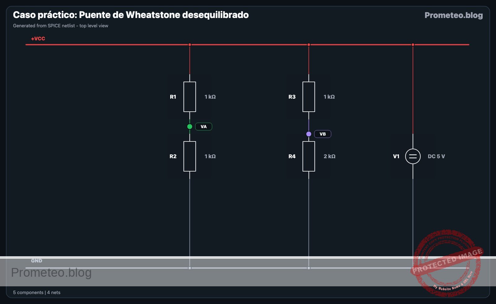
- V1: 5 V DC voltage source, function: main power supply.
- R1: 1 kΩ resistor, function: upper reference arm.
- R2: 1 kΩ resistor, function: lower reference arm.
- R3: 1 kΩ resistor, function: upper measurement arm.
- R4: 2 kΩ potentiometer (linear), function: variable resistor (simulating a sensor like a thermistor or strain gauge).
Wiring guide
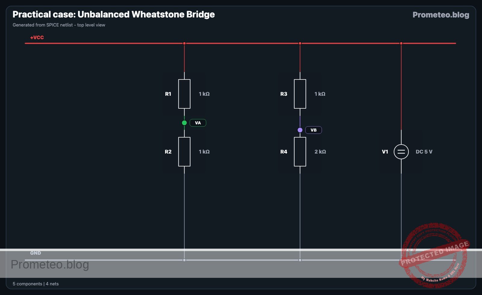
This circuit consists of two parallel voltage dividers connected to a common source. The output is taken differentially between the center points of these dividers.
- V1 connects between node
VCC(positive) and node0(GND). - R1 connects between node
VCCand nodeVA(Reference Point). - R2 connects between node
VAand node0. - R3 connects between node
VCCand nodeVB(Measurement Point). - R4 connects between node
VBand node0. - Measurement: The output VOUT is measured between node
VAand nodeVB.
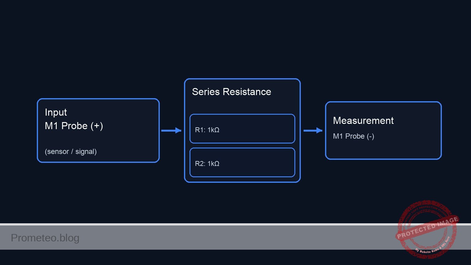
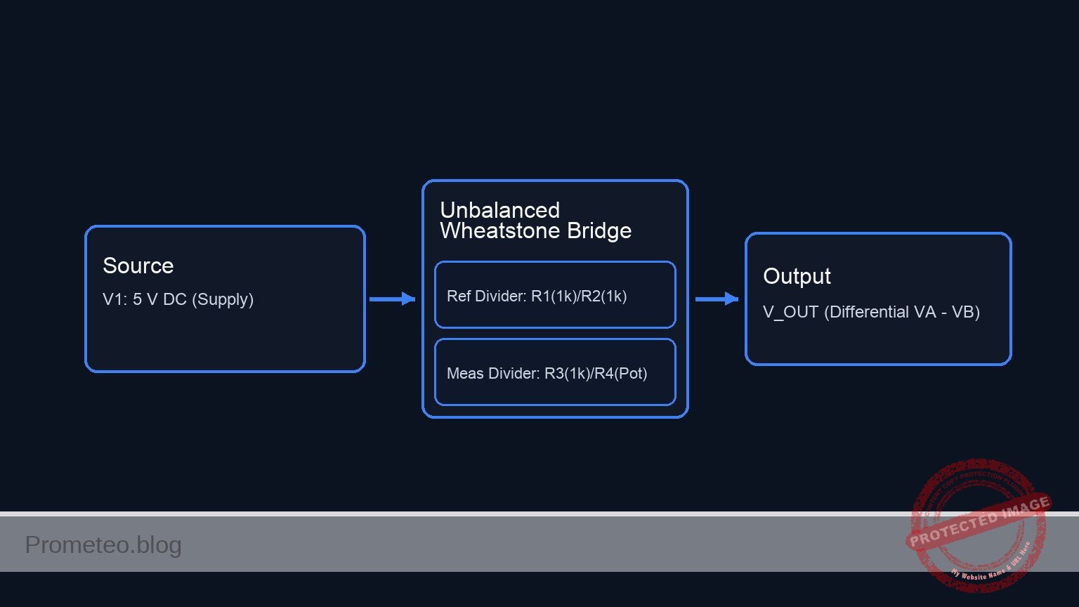
Conceptual block diagram
Schematic
[ SOURCE ]                     [ BRIDGE PROCESSING ]                     [ OUTPUT ]

                               +-----------------------------+
                               |   Reference Divider (Left)  |
                            +->|  (Fixed Ratio: R1 / R2)     |--(Node VA)-->+
                            |  |  [ R1: 1 kΩ ] + [ R2: 1 kΩ ]  |              |
                            |  +-----------------------------+              |
                            |                                               v
[ V1: 5 V DC ] --(Supply)--> +                                          [ V_OUT ]
                            |                                          (Differential)
                            |  +-----------------------------+         ( VA - VB )
                            |  |  Measurement Divider (Right)|              ^
                            +->|  (Variable Ratio: R3 / R4)  |--(Node VB)-->+
                               |  [ R3: 1 kΩ ] + [ R4: Pot ]  |
                               +-----------------------------+
Electrical diagram
Measurements and tests
Follow these steps to validate the bridge operation using a voltmeter or multimeter.
- Setup: Power the circuit with 5 V. Set your multimeter to measure DC Voltage in the 20 V or 2 V range.
- Verify Reference: Measure the voltage between
VAand0(GND). With R1 and R2 being equal (1 kΩ), this should be stable at exactly 2.5 V. - Find the Null Point: Connect the multimeter probes between
VA(red probe) andVB(black probe). Adjust potentiometer R4 until the multimeter reads 0.00 V.- Observation: At this point, the bridge is balanced (R1 / R2 = R3 / R4). R4 should be approximately 1 kΩ.
- Simulate Sensor Increase: Increase the resistance of R4.
- Observation: The voltage at
VBrises. The differential reading (VA – VB) will become negative (assuming Red probe on A, Black on B).
- Observation: The voltage at
- Simulate Sensor Decrease: Decrease the resistance of R4 below 1 kΩ.
- Observation: The voltage at
VBdrops. The differential reading will become positive.
- Observation: The voltage at
SPICE netlist and simulation
Reference SPICE Netlist (ngspice) — excerptFull SPICE netlist (ngspice)
* Practical case: Unbalanced Wheatstone Bridge

* --- Power Supply ---
* V1: 5 V DC voltage source, main power supply
V1 VCC 0 DC 5

* --- Reference Arm (Left) ---
* R1: 1 kΩ, upper reference arm
R1 VCC VA 1k

* R2: 1 kΩ, lower reference arm
R2 VA 0 1k

* --- Measurement Arm (Right) ---
* R3: 1 kΩ, upper measurement arm
R3 VCC VB 1k

* R4: 2 kΩ potentiometer (simulating sensor), lower measurement arm
* Connected between VB and 0. Set to 2k to demonstrate unbalanced state.
R4 VB 0 2k
* ... (truncated in public view) ...
Copy this content into a .cir file and run with ngspice.
* Practical case: Unbalanced Wheatstone Bridge

* --- Power Supply ---
* V1: 5 V DC voltage source, main power supply
V1 VCC 0 DC 5

* --- Reference Arm (Left) ---
* R1: 1 kΩ, upper reference arm
R1 VCC VA 1k

* R2: 1 kΩ, lower reference arm
R2 VA 0 1k

* --- Measurement Arm (Right) ---
* R3: 1 kΩ, upper measurement arm
R3 VCC VB 1k

* R4: 2 kΩ potentiometer (simulating sensor), lower measurement arm
* Connected between VB and 0. Set to 2k to demonstrate unbalanced state.
R4 VB 0 2k

* --- Simulation Setup ---
* Calculate DC operating point
.op

* Transient analysis (10ms duration to verify stability)
.tran 100u 10m

* --- Output Directives ---
* Monitor Supply, Reference Voltage (VA), and Sensor Voltage (VB)
* Differential Output VOUT = V(VA) - V(VB)
.print tran V(VCC) V(VA) V(VB)

.end
Simulation Results (Transient Analysis)

Show raw data table (108 rows)
Index   time            v(vcc)          v(va)           v(vb)
0	0.000000e+00	5.000000e+00	2.500000e+00	3.333333e+00
1	1.000000e-06	5.000000e+00	2.500000e+00	3.333333e+00
2	2.000000e-06	5.000000e+00	2.500000e+00	3.333333e+00
3	4.000000e-06	5.000000e+00	2.500000e+00	3.333333e+00
4	8.000000e-06	5.000000e+00	2.500000e+00	3.333333e+00
5	1.600000e-05	5.000000e+00	2.500000e+00	3.333333e+00
6	3.200000e-05	5.000000e+00	2.500000e+00	3.333333e+00
7	6.400000e-05	5.000000e+00	2.500000e+00	3.333333e+00
8	1.280000e-04	5.000000e+00	2.500000e+00	3.333333e+00
9	2.280000e-04	5.000000e+00	2.500000e+00	3.333333e+00
10	3.280000e-04	5.000000e+00	2.500000e+00	3.333333e+00
11	4.280000e-04	5.000000e+00	2.500000e+00	3.333333e+00
12	5.280000e-04	5.000000e+00	2.500000e+00	3.333333e+00
13	6.280000e-04	5.000000e+00	2.500000e+00	3.333333e+00
14	7.280000e-04	5.000000e+00	2.500000e+00	3.333333e+00
15	8.280000e-04	5.000000e+00	2.500000e+00	3.333333e+00
16	9.280000e-04	5.000000e+00	2.500000e+00	3.333333e+00
17	1.028000e-03	5.000000e+00	2.500000e+00	3.333333e+00
18	1.128000e-03	5.000000e+00	2.500000e+00	3.333333e+00
19	1.228000e-03	5.000000e+00	2.500000e+00	3.333333e+00
20	1.328000e-03	5.000000e+00	2.500000e+00	3.333333e+00
21	1.428000e-03	5.000000e+00	2.500000e+00	3.333333e+00
22	1.528000e-03	5.000000e+00	2.500000e+00	3.333333e+00
23	1.628000e-03	5.000000e+00	2.500000e+00	3.333333e+00
... (84 more rows) ...
Common mistakes and how to avoid them
- Measuring relative to Ground: Students often measure
VAto GND andVBto GND separately. While valid, the bridge is designed to be measured differentially (VAtoVB) directly.- Solution: Place the voltmeter probes directly across the bridge midpoints.
- Using low-tolerance resistors: If R1 and R2 have high tolerance (e.g., 10%), the reference voltage
VAwill not be exactly VCC/2, making the null point hard to calculate.- Solution: Use 1% metal film resistors for R1, R2, and R3 for precision.
- Loading the bridge: Connecting a low-impedance load (like a motor or a low-resistance speaker) directly between
VAandVB.- Solution: The bridge is for signal measurement, not power. Always connect the output nodes to a high-impedance input, such as an Op-Amp or microcontroller ADC.
Troubleshooting
- Symptom: Output voltage is always 0 V regardless of potentiometer position.
- Cause: Power supply is off or there is a short circuit between
VAandVB. - Fix: Check V1 connections and ensure the two legs of the bridge are not shorted together.
- Cause: Power supply is off or there is a short circuit between
- Symptom: Cannot reach 0 V (Null point) output.
- Cause: The fixed resistor R3 is significantly different from the range of potentiometer R4.
- Fix: Ensure R4’s range includes the value of R3 (e.g., if R3 is 1 kΩ, R4 must be capable of reaching 1 kΩ).
- Symptom: Readings are unstable or «jittery».
- Cause: Noisy potentiometer wiper or loose breadboard contacts.
- Fix: Replace the potentiometer or ensure solid connections on the breadboard.
Possible improvements and extensions
- Instrumentation Amplifier: Feed nodes
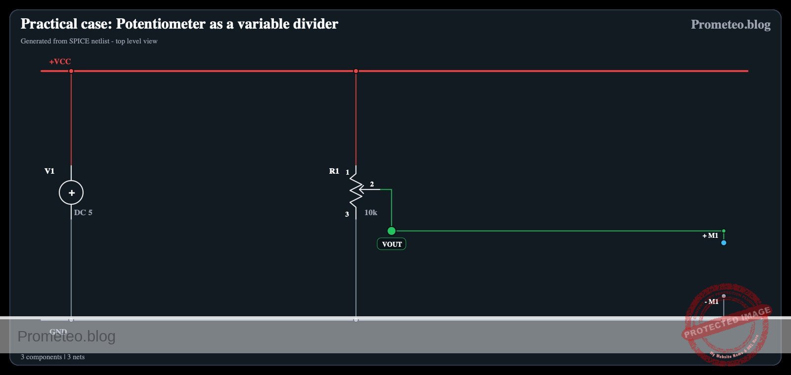
VAandVBinto an instrumentation amplifier (like the AD620) to amplify the small differential voltage for a microcontroller to read. - Physical Sensor: Replace R4 with a photoresistor (LDR) or a thermistor (NTC). Observe how light or temperature changes the bridge balance.
More Practical Cases on Prometeo.blog
Find this product and/or books on this topic on Amazon
As an Amazon Associate, I earn from qualifying purchases. If you buy through this link, you help keep this project running.
Quick Quiz

Telecommunications Electronics Engineer and Computer Engineer (official degrees in Spain).